Start Trading Now
Sign up for ZitaPlus, where knowledge and personalized support come together for your success.
Open Real Account Open Demo Account
Expected Shortfall, often abbreviated as ES and also known as Conditional Value at Risk (CVaR) or Expected Tail Loss, is an advanced risk metric used to quantify the expected loss of a portfolio in extreme market conditions. In simple terms, Expected Shortfall answers a fundamental question: When our bad days turn into absolute disasters, how much money should we expect to lose on average?
Unlike traditional metrics that only identify the entry threshold of a crisis, Expected Shortfall looks directly into the tail end of a loss distribution. It calculates the average of all potential losses that exceed a chosen risk boundary, providing risk managers with a clearer picture of structural exposure.
Risk Threshold (VaR Cutoff) ──► Tail Loss Distribution ──► Average of Extreme Losses (Expected Shortfall)
To grasp how Expected Shortfall works, it helps to understand its mathematical relationship with standard Value at Risk (VaR). While VaR acts as a static cutoff line, Expected Shortfall takes the integral of all outcomes beyond that line.
Mathematically, if X represents the loss distribution of a portfolio over a specific time horizon, and a represents the target confidence level (such as 95% or 99%), Expected Shortfall is formally defined as:
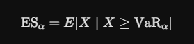
In this equation, VaRa represents the Value at Risk at confidence level a, and E[.] denotes the expected value (or mathematical average).
When working with continuous probability distributions where the loss variable has a smooth density function f(x), Expected Shortfall can be expressed in continuous terms:
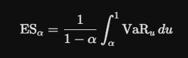
This formula shows that Expected Shortfall is literally the mathematical average of all VaR values calculated at every confidence level between a and 100%. If your confidence level is 97.5%, the calculation averages every possible loss outcome sitting in that worst 2.5% tail.
For many years, Value at Risk was the undisputed benchmark for institutional risk management. However, severe regulatory flaws in standard VaR became undeniable during major global market disruptions.
Value at Risk is inherently blind to tail depth. Suppose a trading desk has a 1-day 99% VaR of $1 million. That figure tells you there is a 1% chance the desk will lose more than $1 million tomorrow. However, it completely fails to explain whether that 1% event will cost $1.1 million or $100 million.
This blind spot created dangerous incentives. Financial institutions could design portfolios that stayed just under their VaR threshold while taking on massive, unmonitored tail risk that could trigger insolvency during a market panic.
In academic risk theory, a reliable risk metric must be coherent. One key requirement of a coherent risk metric is subadditivity, which mathematically states that the total risk of a combined portfolio should never exceed the sum of the risks of its individual parts:
Risk (A+B) < Risk (A) + Risk (B)
Standard VaR fails the subadditivity test under many market conditions, meaning combining two diversified portfolios can sometimes yield a higher VaR than holding them separately. Expected Shortfall, by contrast, is mathematically proven to be coherent and subadditive under all conditions. It always honors the benefits of portfolio diversification.
Individual Portfolio Risks ──► Combined Portfolio ──► Guaranteed Lower or Equal Risk (Subadditivity)
Because of these mathematical properties, global banking regulators under the Basel III framework officially shifted their market risk requirements away from 99% VaR in favor of a 97.5% Expected Shortfall metric.
Risk analysts generally use three main approaches to calculate Expected Shortfall, matching the methods used in traditional portfolio modeling.
The historical method takes raw past return data over a set period, such as 500 trading days, and applies those return percentages to the current portfolio.
If you analyze 1,000 historical days at a 97.5% confidence level, the worst 2.5% represents 25 days. Your Expected Shortfall is simply the average loss of those 25 worst days.
The parametric method assumes that asset returns follow a known statistical distribution, such as a normal curve or a Student's t-distribution. If returns are assumed to be normally distributed with mean $\mu$ and standard deviation $\sigma$, Expected Shortfall can be calculated using the probability density function and cumulative distribution function.
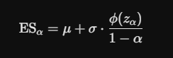
Where Za is the critical value corresponding to the confidence level a. While computationally fast, this method can underestimate risk if the assumed distribution ignores real-world fat tails.
For complex portfolios containing exotic options or non-linear derivatives, risk teams run Monte Carlo simulations. A computer algorithm generates thousands of hypothetical future market scenarios based on key statistical inputs. The portfolio is revalued under every scenario, creating a vast distribution of prospective profits and losses from which the tail average is calculated.
| Method | Best Used For | Primary Benefit | Potential Drawback |
| Historical | Portfolios with simple assets | No theoretical distribution assumptions | Bound strictly by past events |
| Parametric | Linear portfolios with stable data | Fast execution and low computing load | Vulnerable to non-normal distributions |
| Monte Carlo | Complex derivatives & structured debt | Models dynamic asset interactions | Requires immense computing power |
Expected Shortfall is not just a theoretical equation for regulatory filings. It directly shapes how institutional investors manage capital, allocate assets, and hedge downside risks.
Investment banks use Expected Shortfall to assign capital requirements to individual trading desks. Desks that trade volatile, illiquid instruments like high-yield corporate credit or emerging market currencies carry larger tail risks. A high Expected Shortfall calculation forces the firm to set aside larger cash buffers against those desks, keeping overall leverage under control.
Portfolio managers regularly combine Expected Shortfall with deterministic stress testing. During macro uncertainties, managers simulate severe historical shocks, like liquidity crunches or sharp interest rate hikes, to evaluate how bad the average loss inside the extreme tail would be. This allows them to build dynamic hedging strategies using put options or index futures before market stress hits.
While Expected Shortfall is a vast improvement over basic VaR, it comes with its own set of operational challenges.
Validating a risk model through historical backtesting is crucial for institutional accuracy. Testing a standard VaR model is straightforward: you simply count how many times actual daily losses breached the predicted threshold over a year.
Backtesting Expected Shortfall is much harder because you are trying to verify an average loss value inside a region that, by definition, rarely produces data points.
Because Expected Shortfall takes an average of all tail losses, a single anomalous outlier in the historical dataset can dramatically skew the final calculation. A single sudden flash crash or policy shock can cause your Expected Shortfall figures to jump overnight, forcing unnecessary portfolio adjustments if the event was an isolated anomaly.
Expected Shortfall provides a realistic framework for evaluating portfolio exposure when markets move beyond normal behavior. By measuring the severity of severe downside outcomes rather than stopping at a basic probability line, it eliminates dangerous blind spots in risk reporting.
Understanding Expected Shortfall allows fund managers and trading operations to build portfolios that can withstand severe market shifts without suffering catastrophic capital depletion.
What is the main difference between VaR and Expected Shortfall?
Value at Risk identifies the minimum threshold loss expected at a specific confidence level, while Expected Shortfall calculates the average magnitude of all losses that exceed that threshold.
Why did Basel III switch from VaR to Expected Shortfall?
Regulators switched because standard VaR failed to capture the depth of severe losses during financial crises and failed to properly account for portfolio diversification benefits under subadditivity rules.
Is Expected Shortfall always larger than Value at Risk?
Yes. Because Expected Shortfall is the average of all loss outcomes extending beyond the VaR cutoff line, its value is mathematically guaranteed to be equal to or greater than the VaR figure for the same confidence level.
What confidence level is typically used for Expected Shortfall?
Under current regulatory standards like Basel III, a 97.5% confidence level is the standard benchmark for Expected Shortfall, replacing the traditional 99% confidence level previously used for Value at Risk.
Can Expected Shortfall completely prevent catastrophic trading losses?
No risk model can prevent losses entirely. Expected Shortfall is an estimation tool based on historical patterns or statistical assumptions, meaning an unprecedented market event can still produce losses that exceed model expectations.
Would like to learn how to look financial markets from a different angle? Then keep reading and invest yourself with ZitaPlus.